

Starting with a clean image x0, we iteratively add noise to generate progressively noisier images xt, until we reach pure noise at timestep t = T. At t = 0, we have a clean image, and for larger t, the image becomes noisier.
A diffusion model reverses this process by denoising the noisy image xt at each timestep. Using the predicted noise, we can either remove all noise to estimate x0 or partially denoise it to get xt-1. The process continues iteratively until we obtain a clean image x0.
To generate new images, the process begins with pure noise sampled from a Gaussian distribution at timestep T, denoted as xT. By progressively denoising, we generate a clean image.
The amount of noise added at each step is determined by noise coefficients αt, predefined during training.
The forward process adds noise to a clean image x0. The process is defined by:
q(xt|x0) = N(xt; √α̅tx0, (1 - α̅t)I)
This is equivalent to:
xt = √α̅tx0 + √(1 - α̅t)ε, where ε ~ N(0, 1).
The forward process involves scaling x0 by √α̅t and adding Gaussian noise scaled by √(1 - α̅t).
To implement this, use the alphas_cumprod variable, which contains α̅t values for all t in the range [0, 999]. Remember:
The forward process is tested using a sample image resized to 64x64. For timesteps t in {250, 500, 750}, the results are displayed.


The noisy images are denoised using gaussian blur filter:


The noisy images are denoised using a pretrained diffusion model with the prompt "a high quality photo":


Diffusion models are designed to denoise iteratively. To achieve this, I could start with noise x1000 at timestep T = 1000, denoise step-by-step until reaching x0. However, this would require running the model 1000 times, which is computationally expensive.
We can speed up the process by skipping steps.
To skip steps, I created a new list of timesteps called strided_timesteps. This list corresponds to the noisiest image at the largest timestep, with strided_timesteps[-1] representing a clean image. A stride of 30 works well, so I used it to construct the list.
On the ith denoising step, I used t = strided_timesteps[i] and denoised to t' = strided_timesteps[i+1]. The formula for this is:

Where:
alphas_cumprod.The results comparison are displayed:


Using the same iterative denoise function, I generated 5 images from scratch by setting i_strat to 0, passing in random noise with the prompt "a hight quality photo":


I implemented Classifier-Free Guidance which could improve the generaed image quality. In CGF, a conditional and unconditional noise estimate are computed, and the final noise estimate is a weighted sum of the two. The weights are determined by the conditional noise estimate using this equation, where εu is the unconditional noise estimate, εc is the conditional noise estimate, and ε is the final noise estimate:

where γ controls the strength of CFG. When γ > 1, the generated images have high quality.
The final noise estimate is used to denoise the image. The results are displayed below:


I started with some original test images, and noise it at different strating index, and force it back onto the image manifold without any conditioning.


I also tested the SDEdit on hand drawn and web images:


For this part, I implemented inpainting in which at each timestep, the generated image xt is modified so that the regions specified by m = 0 match the original image xorig. This adjustment ensures consistency with the original image outside the masked region. The formula for this adjustment is:
xt ← m ˆ xt + (1 - m) ˆ forward(xorig, t)
This means that everything inside the mask (where m is 1) is filled with new content, while the areas outside the mask (where m is 0) remain unchanged, incorporating the appropriate amount of noise for timestep t.
The results are displayed below:


I implemented SDEdit with a different prompt for this part:
1. Prompt "a rocket ship"


2. Prompt "a broccoli"


3. Prompt "a ninja"


Our goal is to generate an image that appears as prompt1 but, when flipped upside down, transforms into the image of a different prompt.
I followed algorithm:
    ε₁ = UNet(x_t, t, p₁)
    ε₂ = flip(UNet(flip(x_t), t, p₂))
    ε = (ε₁ + ε₂) / 2
The results are displayed below:
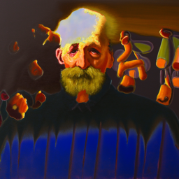
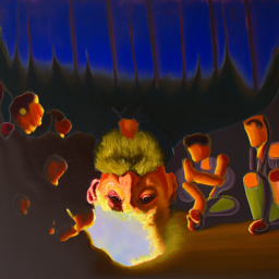
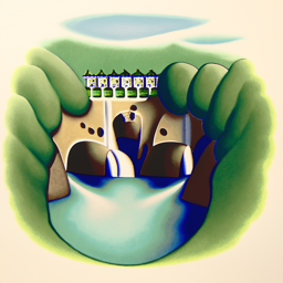
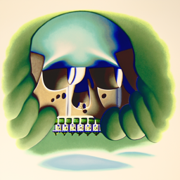
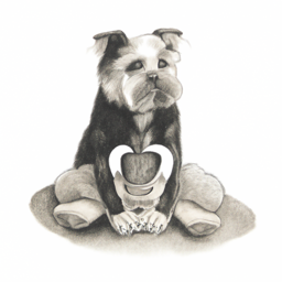
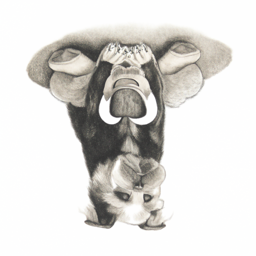
To generate hybrid images using a diffusion model, we will follow a similar approach as described earlier. Specifically, we will estimate the noise using two different text prompts and combine the results to create a composite noise estimate, ε. The composite estimate will merge the low-frequency components from one noise estimate with the high-frequency components from the other. The algorithm is as follows:
        ε₁ = UNet(x_t, t, p₁)
        ε₂ = UNet(x_t, t, p₂)
        ε = f_lowpass(ε₁) + f_highpass(ε₂)




A unconditioned U-Net is implemented to denoise image:
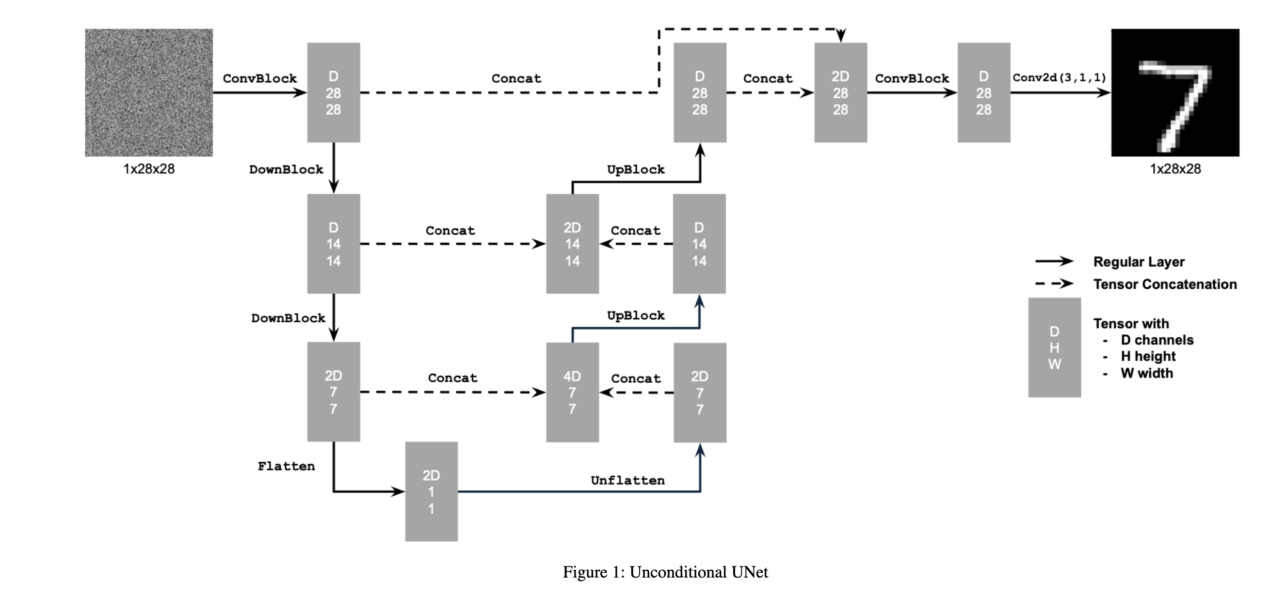
Building on the objective described earlier, our goal is to solve the denoising problem: given a noisy image z, train a denoiser Dθ such that it reconstructs a clean image x. To achieve this, we optimize the following L2 loss function:
L = 𝔼z,x[‖Dθ(z) - x‖²]
To train the denoiser, we generate training pairs (z, x), where each x is a clean MNIST digit. The noisy version z is created by adding Gaussian noise to x as follows:
z = x + σϵ, where ϵ ∼ 𝒩(0, 𝐼)
Here, σ is the noise standard deviation, and ϵ is sampled from a standard normal distribution. We assume that x is normalized in the range [0, 1].
The results of this process for σ values in [0.0, 0.2, 0.4, 0.5, 0.6, 0.8, 1.0] are visualized:
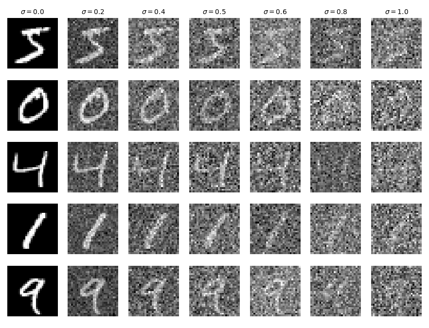
z with σ = 0.5, mapping it to a clean image x.torchvision.datasets.MNIST is used.256.5 epochs.D = 128.1e-4.
L = 𝔼z,x[‖Dθ(z) - x‖²]
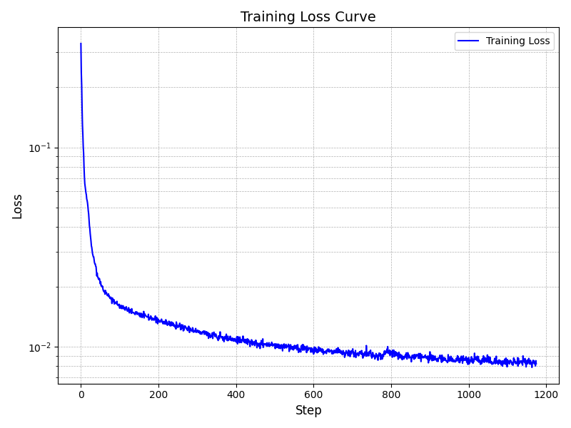
The training loss curve is displayed below, and the model converged at the end of trianing.s
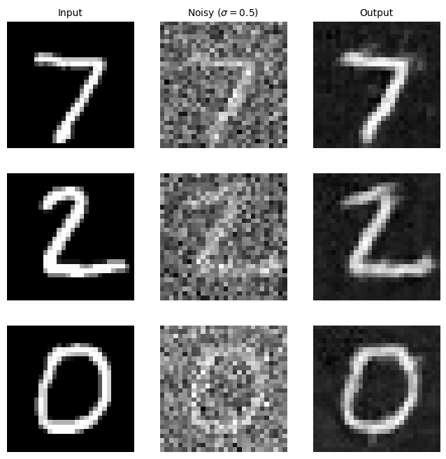
The denoised images sampled from the test set are visualized after epoch 1 and epoch 5. The output after epoch 5 has more defined shapes and less noises.
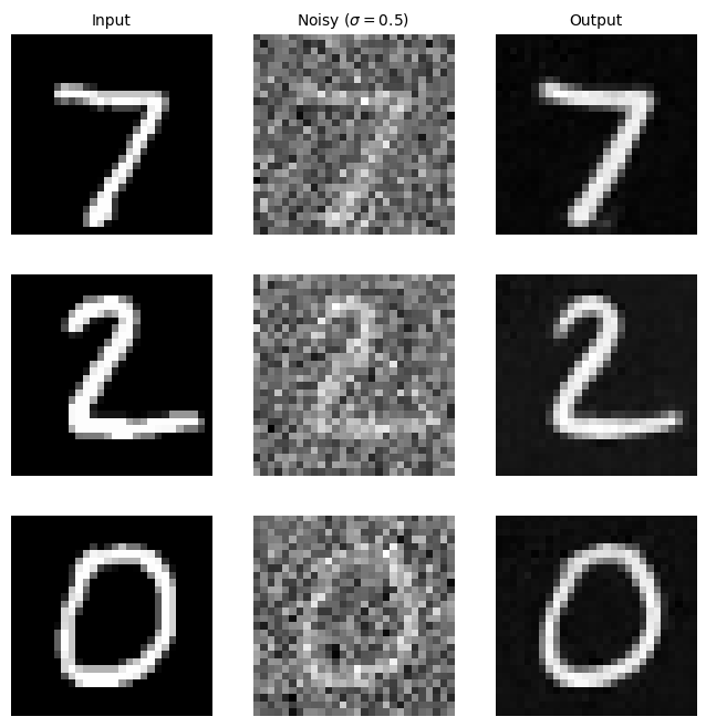
Denoised results are also visualized for out-of-distribution results, denoising images with different σ 's that it wasn't trained for.

In this section, I trained a U-Net model to iteratively denoise images by implementing the Denoising Diffusion Probabilistic Model (DDPM).
Instead of predicting the denoised image, we want the network to predict the noise. Thus, the new objective becomes:
L = 𝔼z,x[‖εθ(z) - ε‖²]
For diffusion, the goal is to start with a pure noise image ε ~ 𝒩(0, I) and iteratively denoise it to generate a realistic image x. We use iterative denoising by sampling noisy images xt for timesteps t ∈ {0, 1, ..., T}, where:
xt = √(α̅t) x0 + √(1 - α̅t) ε
β₀ = 0.0001 and βT = 0.02, with evenly spaced values for other timesteps.
αt = 1 - βt.α̅t = ∏s=1t αsTo denoise xt, we condition the U-Net on the timestep t and minimize loss function:
L = 𝔼xt,x0,t[‖εθ(xt, t) - ε‖²]
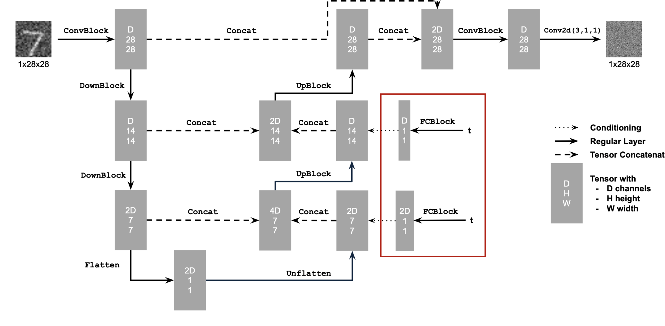
torchvision.datasets.MNIST is used.128.20 epochs.D = 64.1e-3gamma = 0.1^(1.0 / num_epochs)
L = 𝔼xt,x0,t[‖εθ(xt, t) - ε‖²]
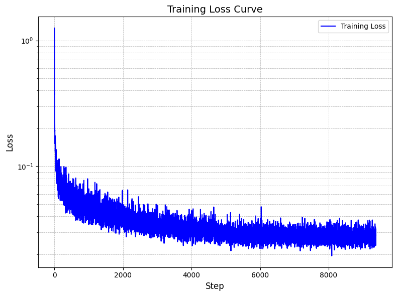
The training loss curve is displayed below
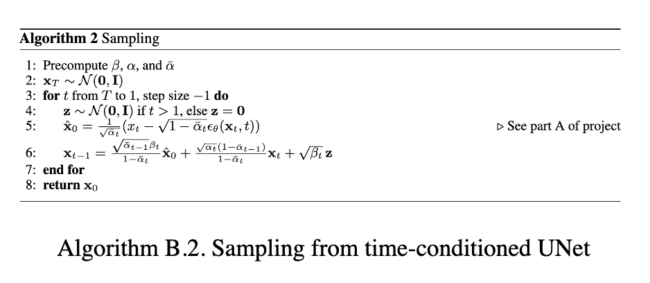
The sampling function is implemented according to the DDPM paper:
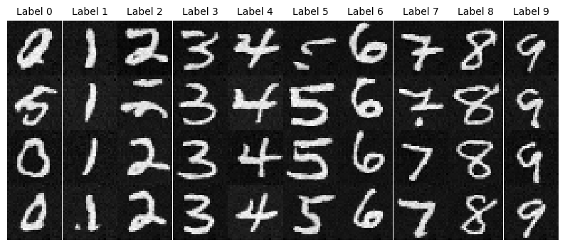
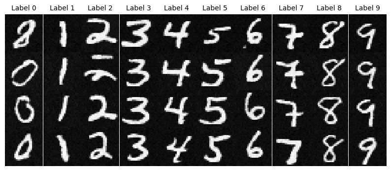
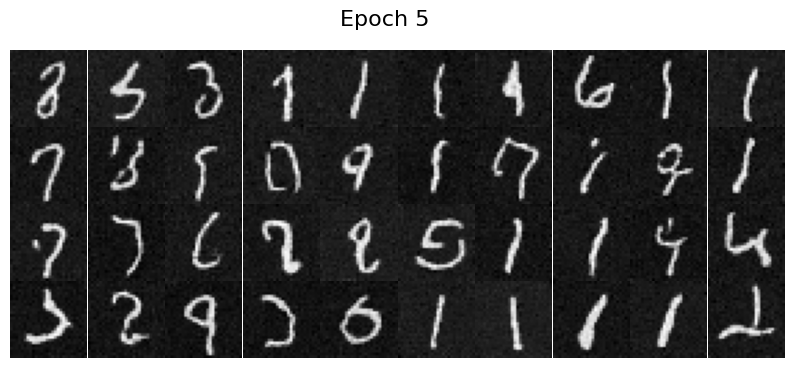
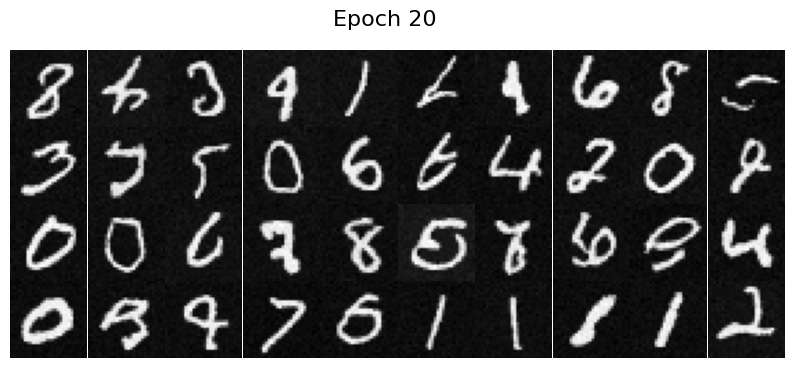
The generated images after epoch 5 and epoch 20 are displayed. The output after epoch 20 has more defined shapes and less noises.
To improve results and provide more control over image generation, we can condition the U-Net on the class of the digit (0–9). Some modifications are implemented on top of the implemention for time conditional U net:
t and the class-conditioning vector c as inputs.puncond = 0.1), set the class-conditioning vector c to zero.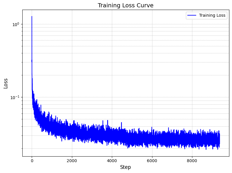
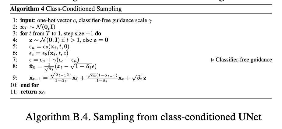
A classifier-free guidance(γ = 0.5) sampling function is implemented according to the DDPM paper:
The generated images after epoch 5 and epoch 20 are displayed. The output after epoch 20 has more defined shapes and less noises.
