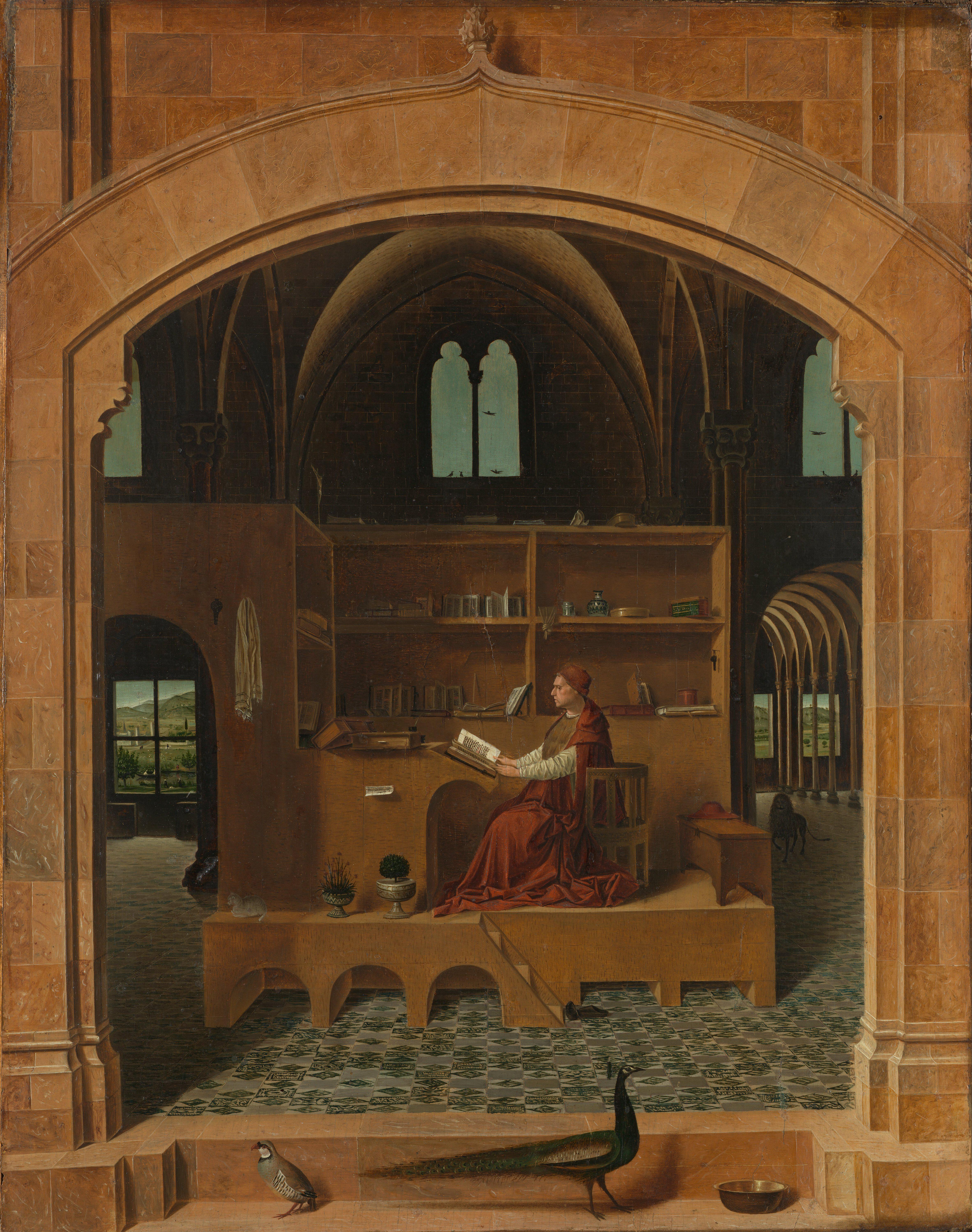
First I create the function computeH() to recover the homography matrix between image 1 and image 2.
The homography matrix \( H \) is given as:
$$ H = \begin{bmatrix} a & b & c \\ d & e & f \\ g & h & i \end{bmatrix} $$
The transformation equation is:
$$ \begin{bmatrix} wx' \\ wy' \\ w \end{bmatrix} = \begin{bmatrix} a & b & c \\ d & e & f \\ g & h & i \end{bmatrix} \begin{bmatrix} x \\ y \\ 1 \end{bmatrix} $$
This expands to two equations for each point correspondence \((x, y) \rightarrow (x', y')\):
$$ x' = \frac{ax + by + c}{gx + hy + 1} $$
$$ y' = \frac{dx + ey + f}{gx + hy + 1} $$
After some rearraning, the equation for solving the homography matrix can be written as:
$$ \begin{bmatrix} x & y & 1 & 0 & 0 & 0 & -xx' & -yx' \\ 0 & 0 & 0 & x & y & 1 & -xy' & -yy' \end{bmatrix} \begin{bmatrix} a \\ b \\ c \\ d \\ e \\ f \\ g \\ h \end{bmatrix} = \begin{bmatrix} x' \\ y' \end{bmatrix} $$
When there are more than 4 correspondences, we then use the least square method to find the optimal solution.
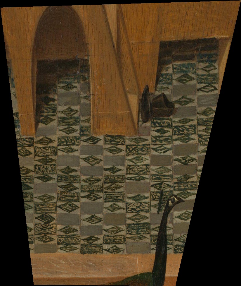
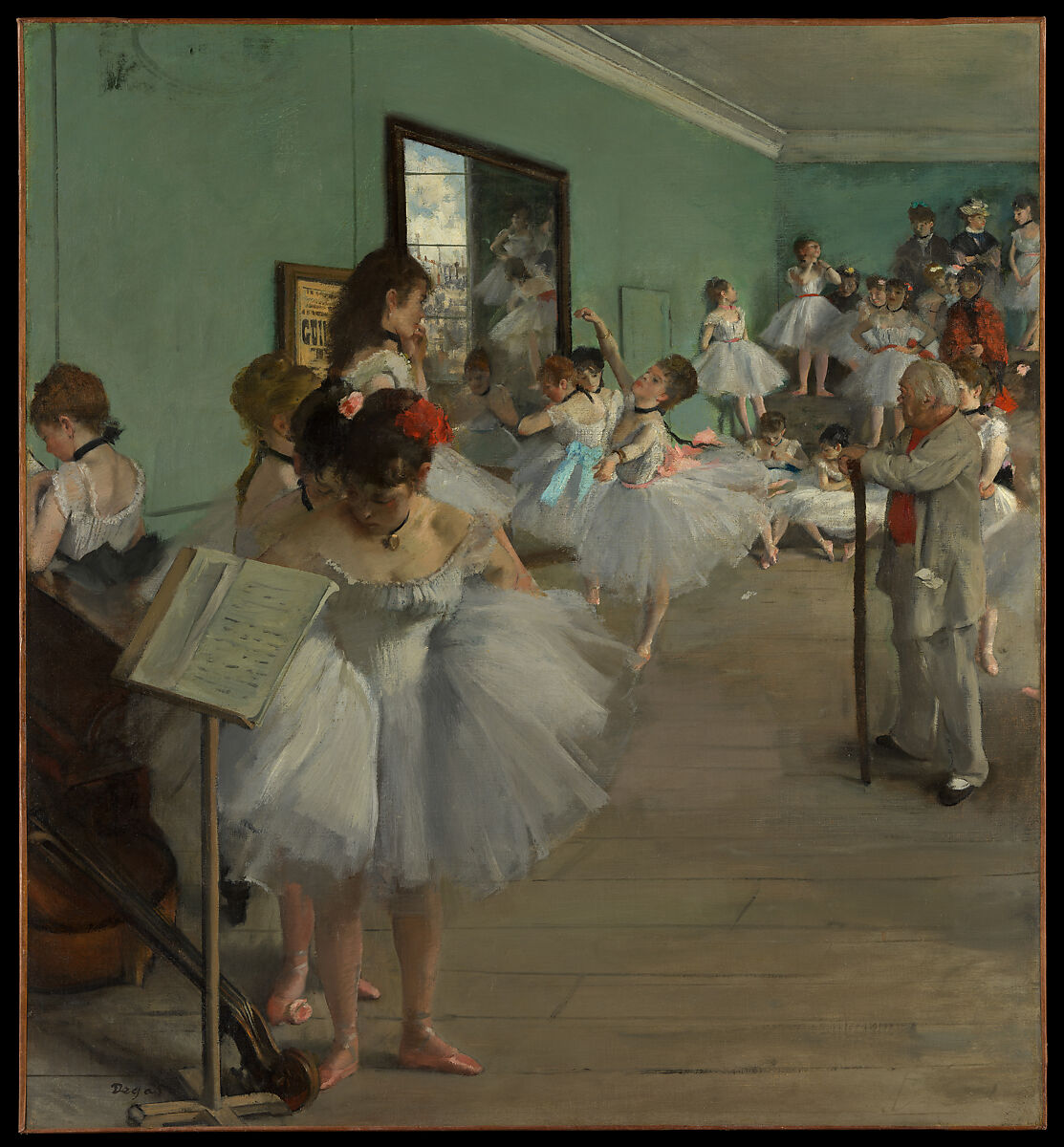
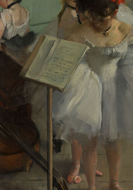
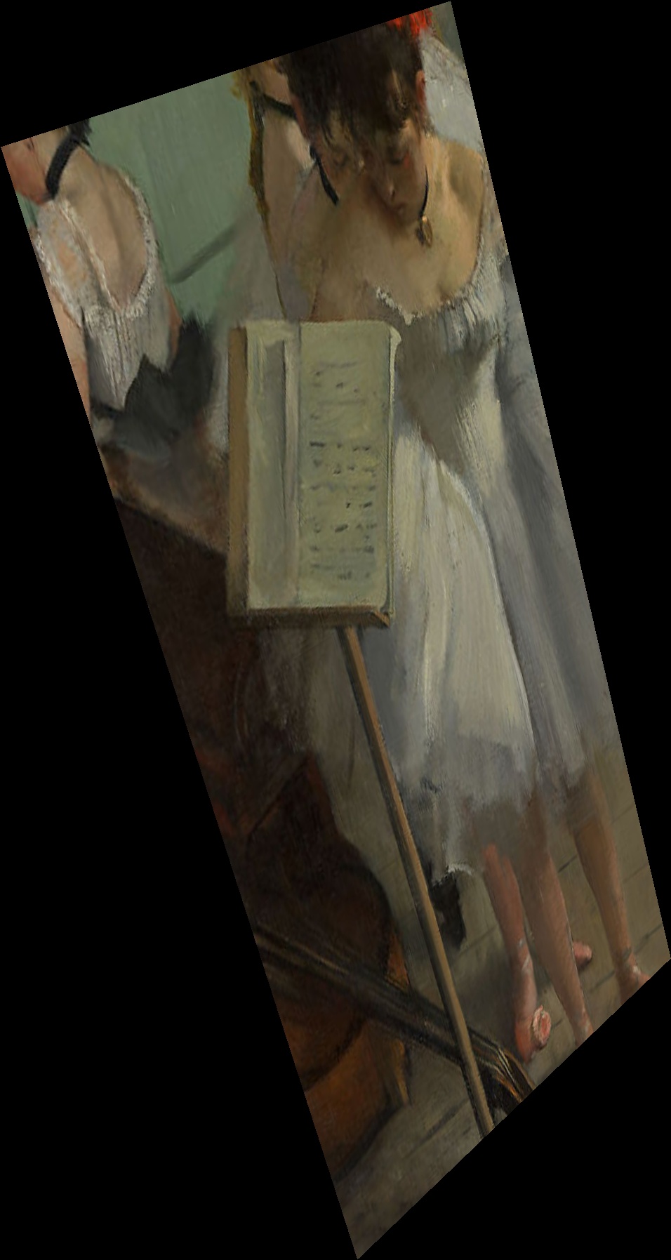
To complete image rectification, I selected the corner of a object in the image that I want to performn rectification, then I manually defined the target rectangular corner coordinate. Then, I found the homography matrix between the two images using these correspondences. Finally, I warped the first image to the rectified perspectives using the homography matrix.
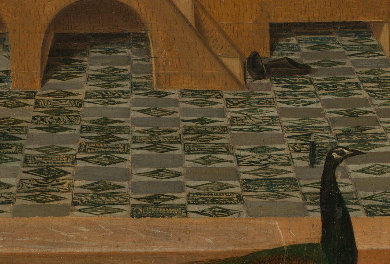
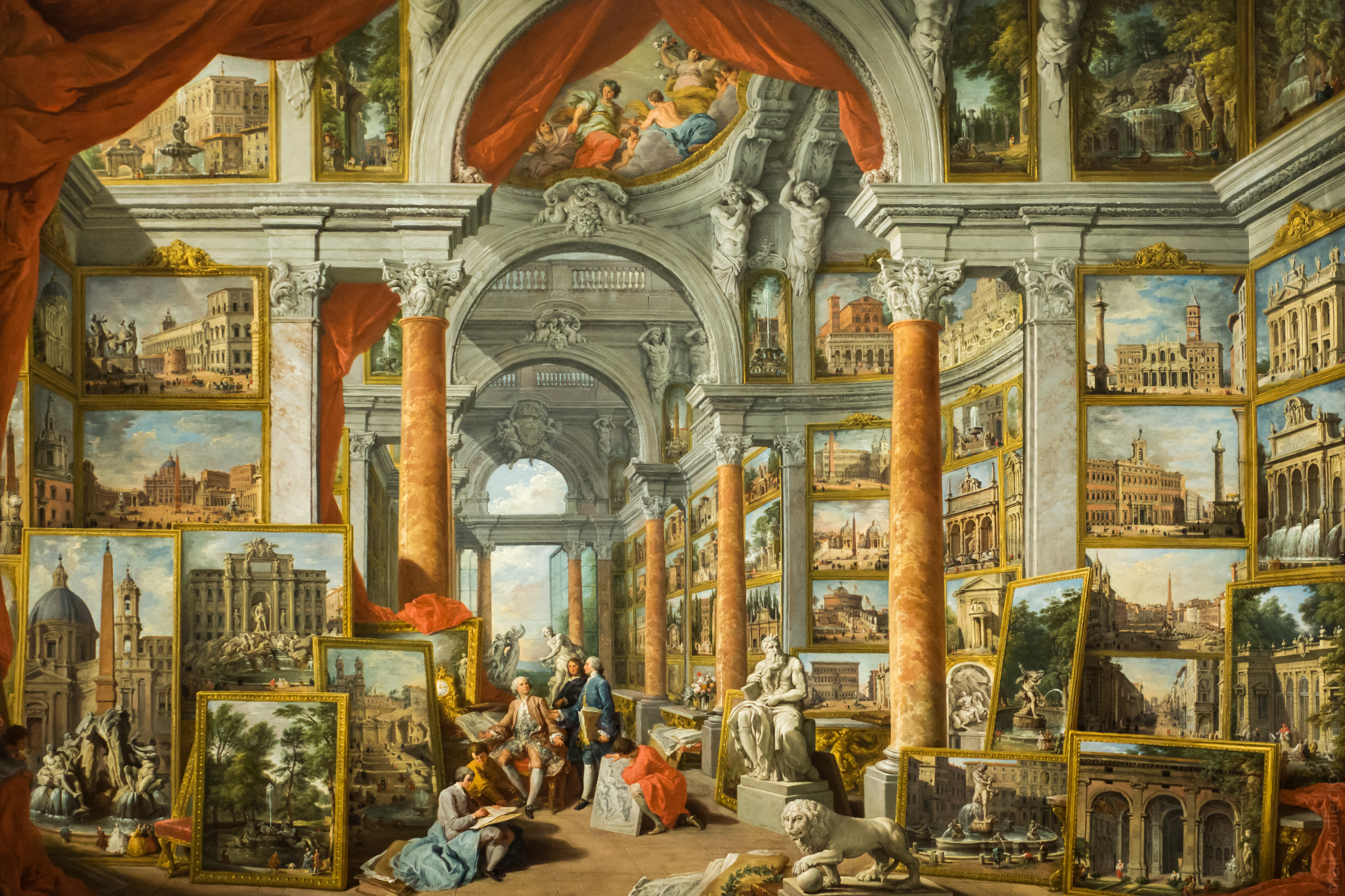
I rectified object appeared in some famous artworks:
1. Floor pattern in the painting: Saint Jerome in His Study by Albrecht Dürer

2. A painting in: Vedute di Roma moderna Giclee by Giovanni Paolo Panini
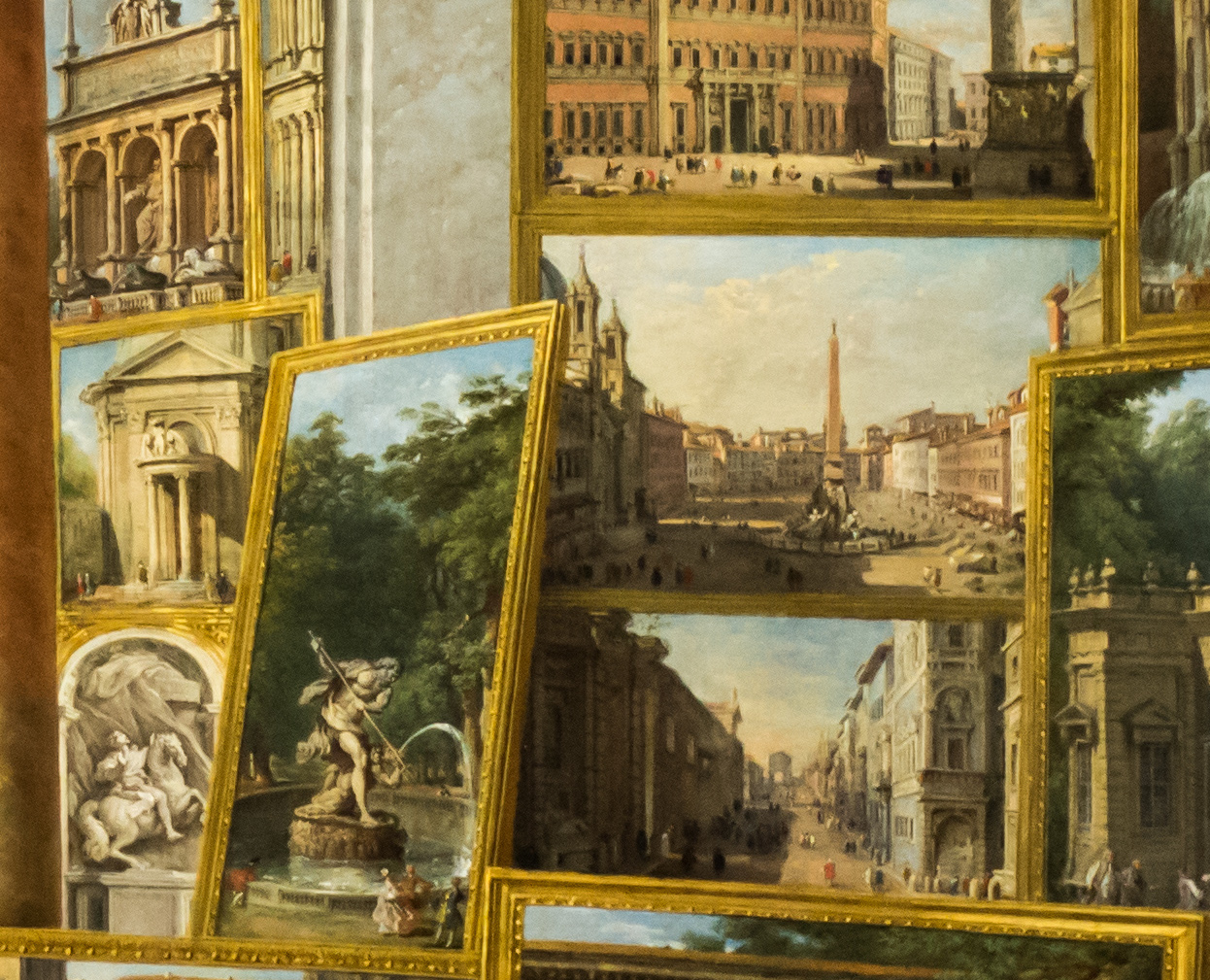
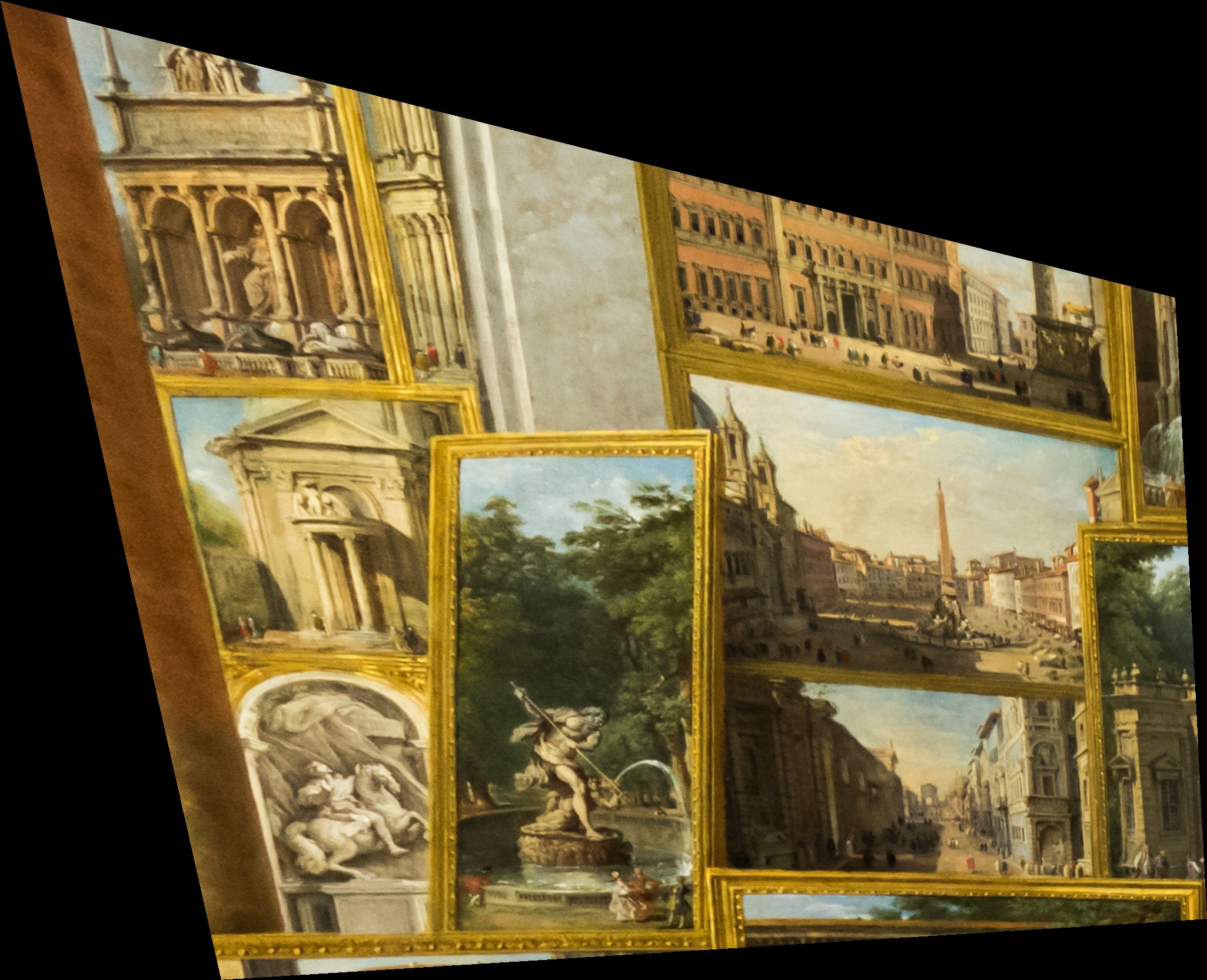
3. Sheet music in The Dance Class by Edgar Degas
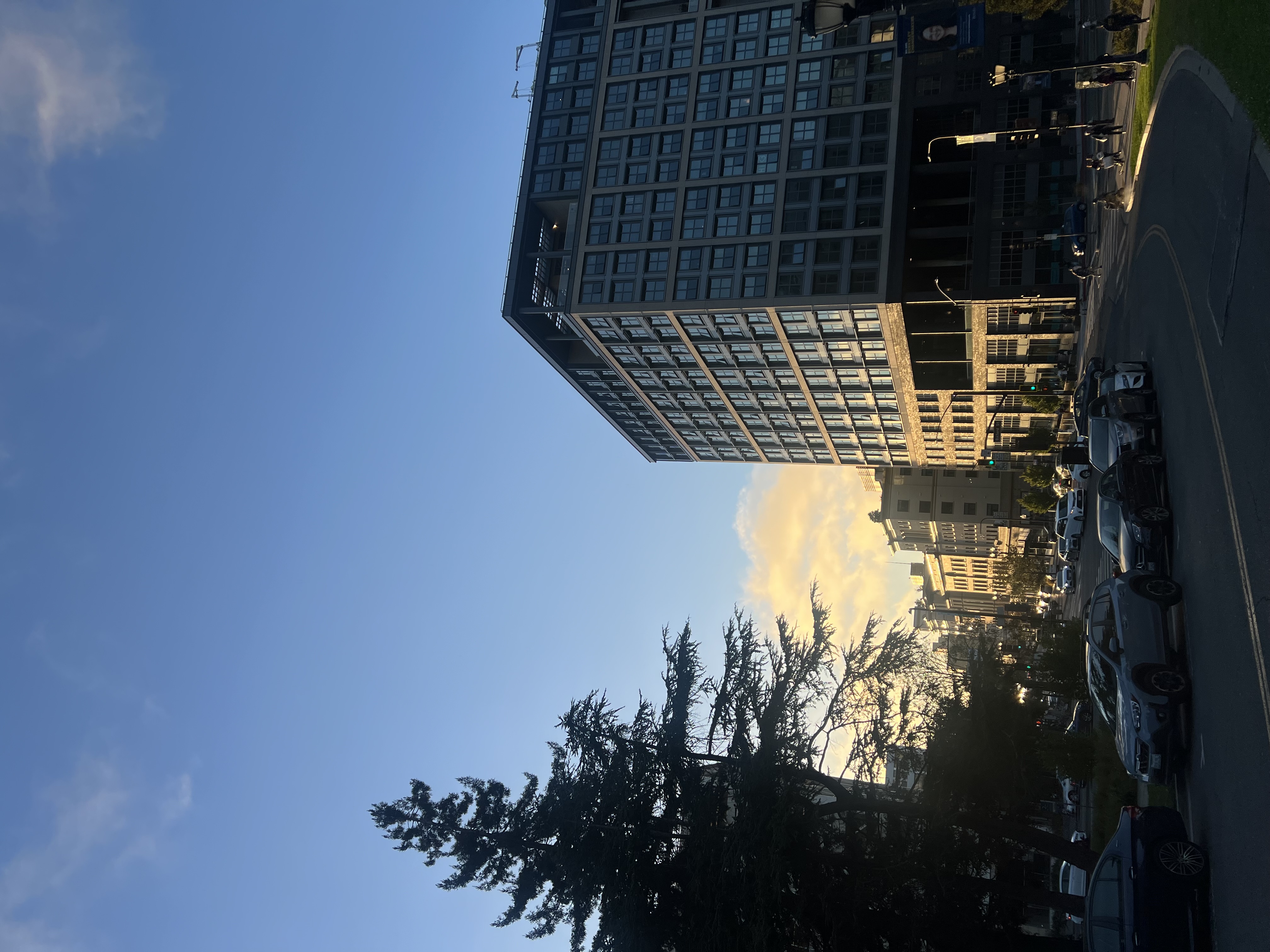
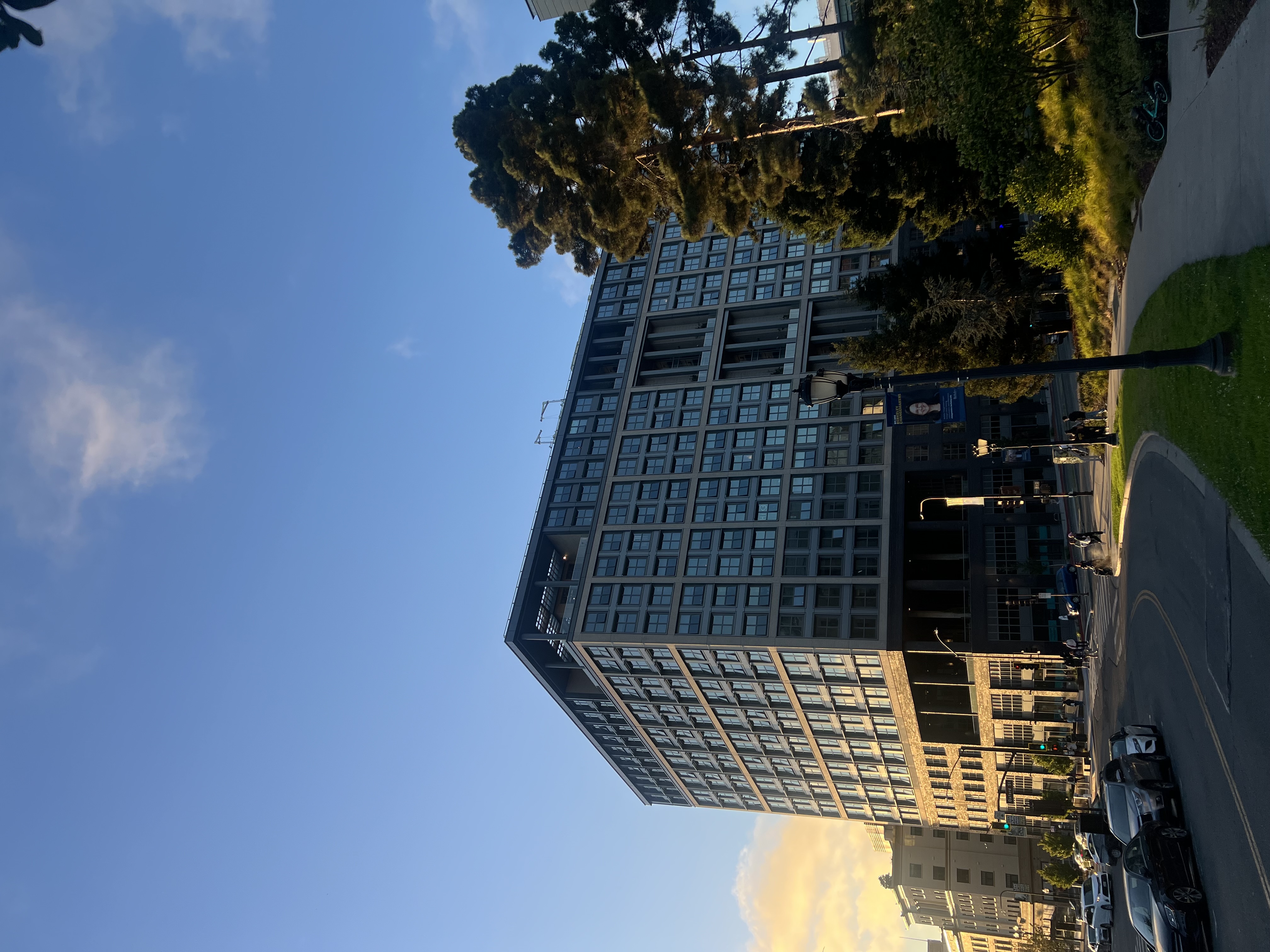
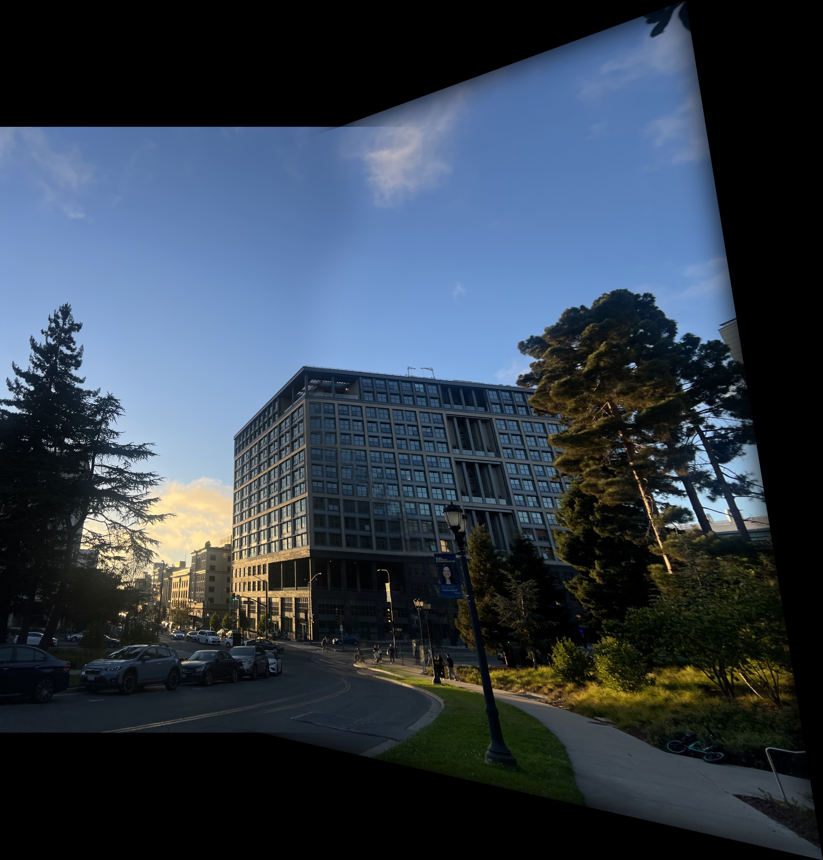
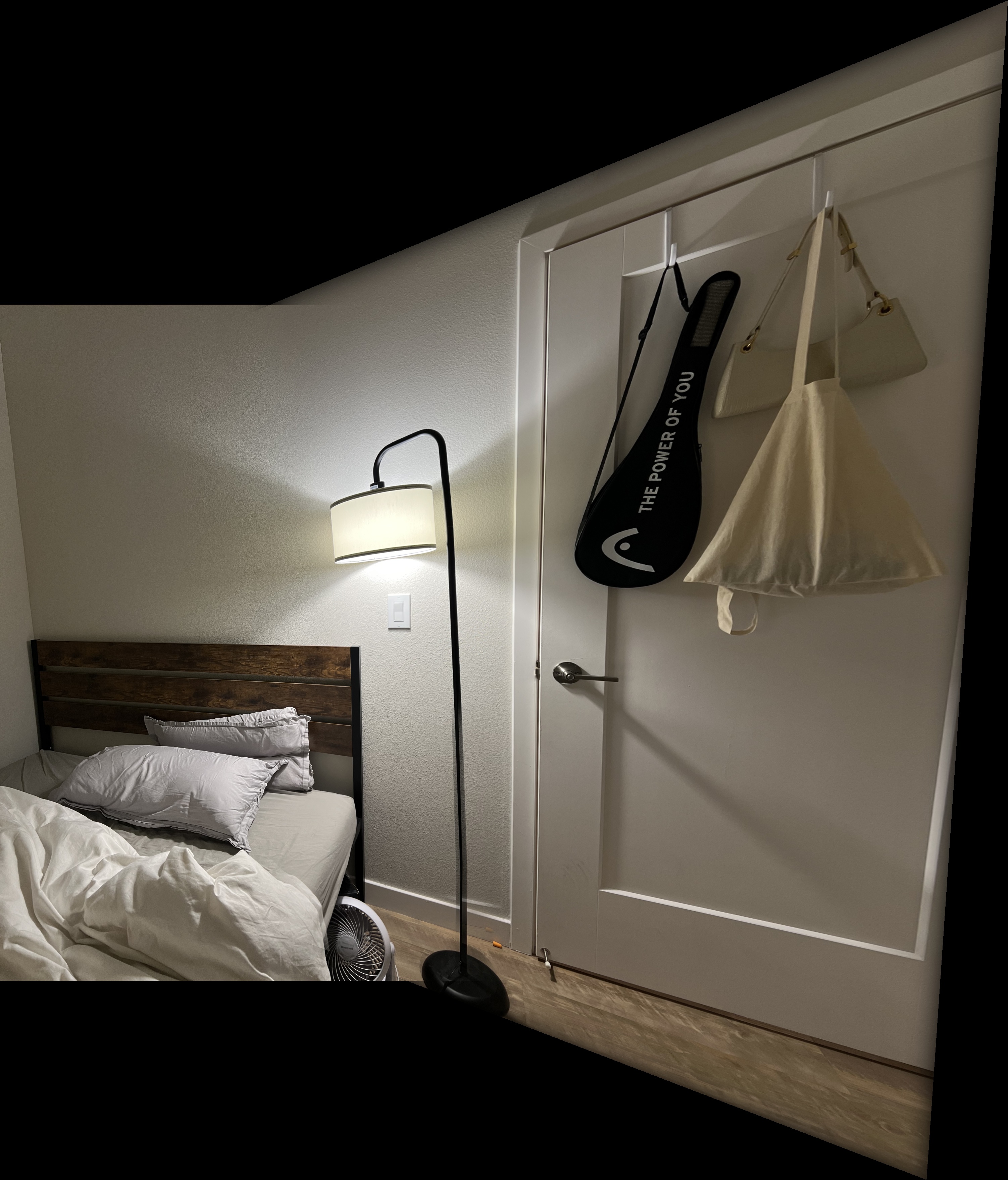
To create a mosaic, I first selected 10 corresponding points in both images and use them to compute the Homography matrix, which aligns image 1 to image 2’s perspective. After warping image 1 using the Homography, I blended the two images using a Gaussian-blurred alpha mask. The distance transform determines each pixel’s proximity to the boundaries of both images, and an alpha mask is created based on these distances. The mask is then smoothed using a Gaussian filter, ensuring a gradual transition between the images. Finally, the images are combined using a linear blend weighted by the alpha mask to produce a smooth mosaic.
Example 1
Example 2
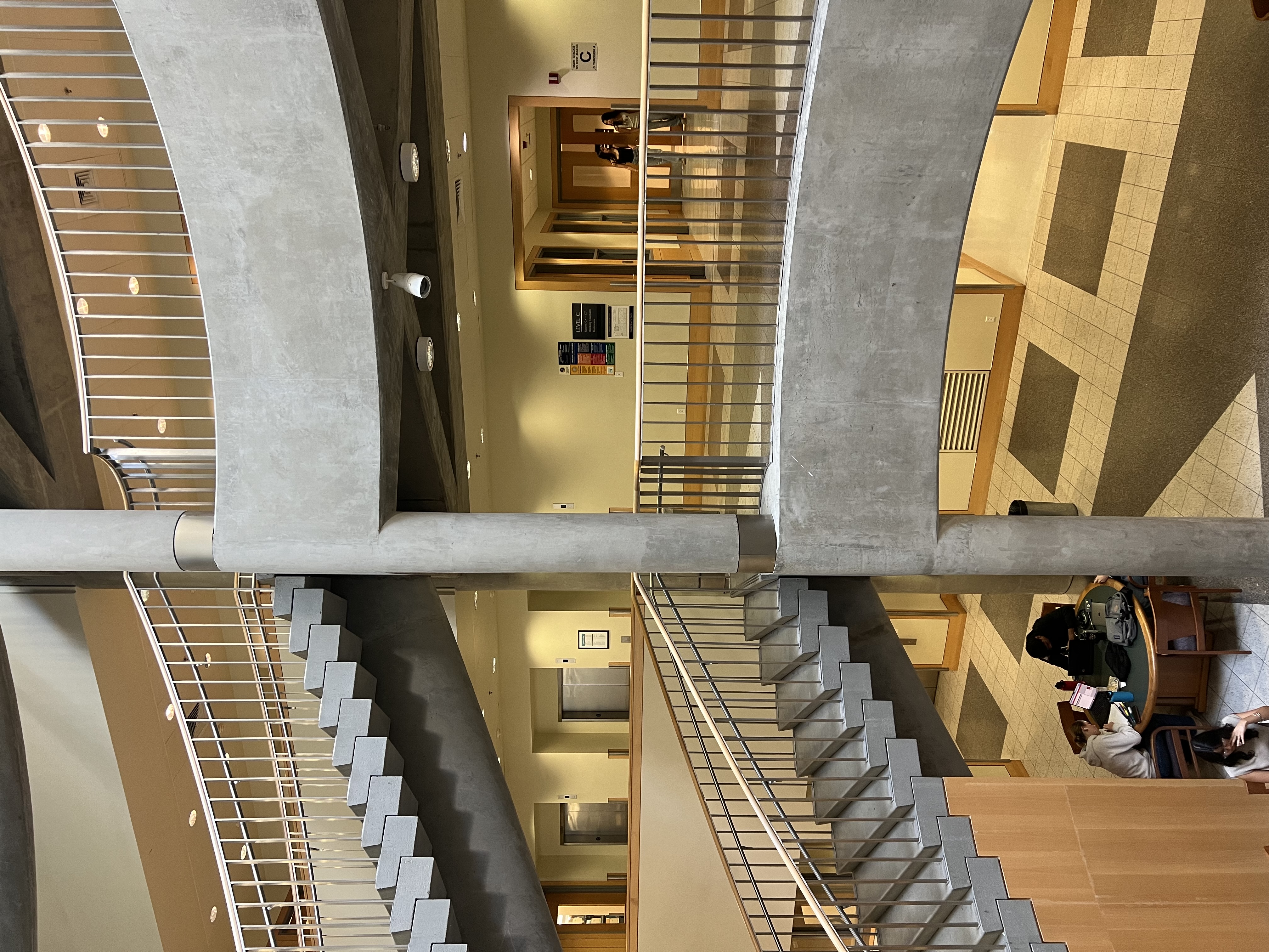
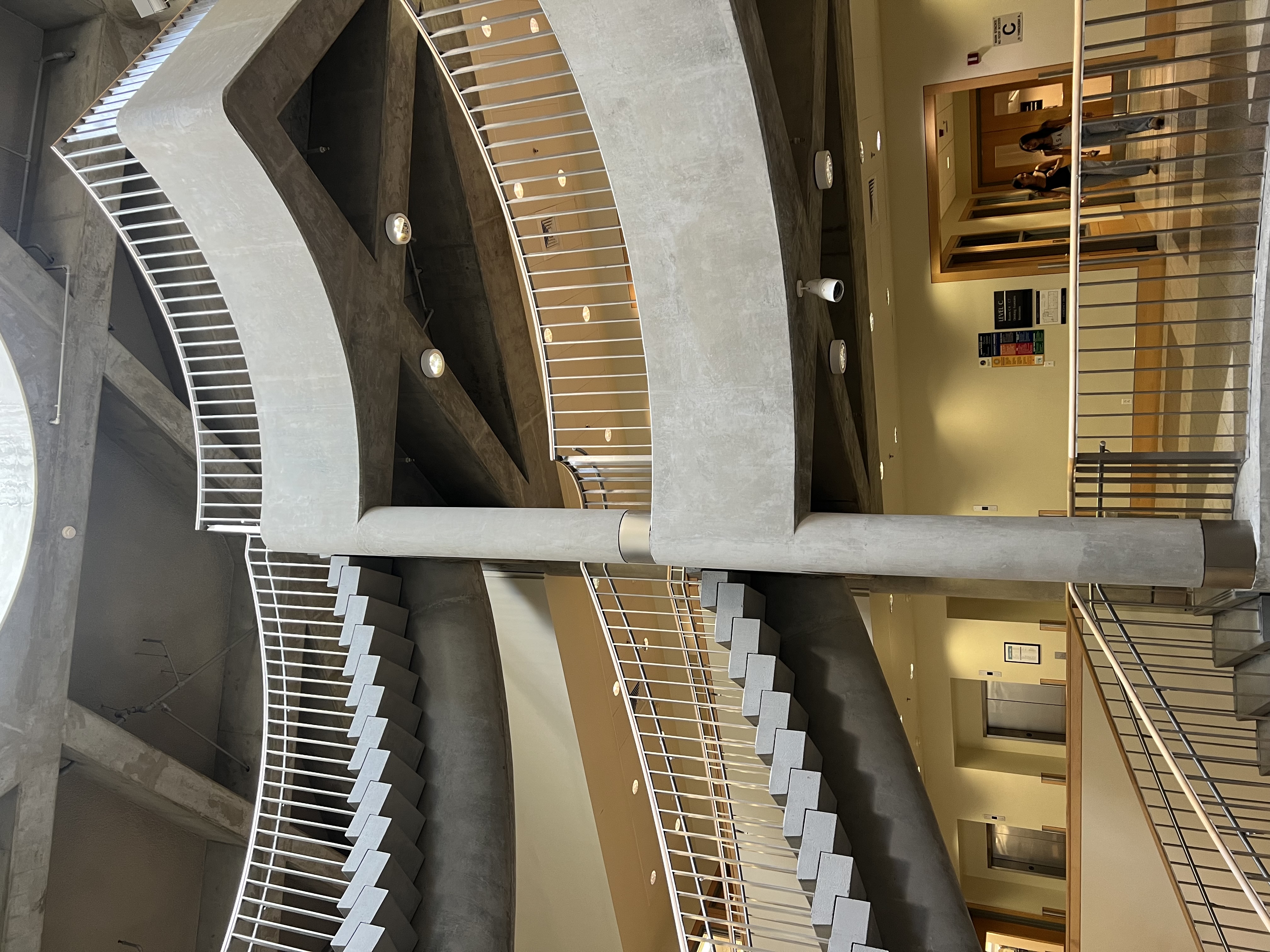
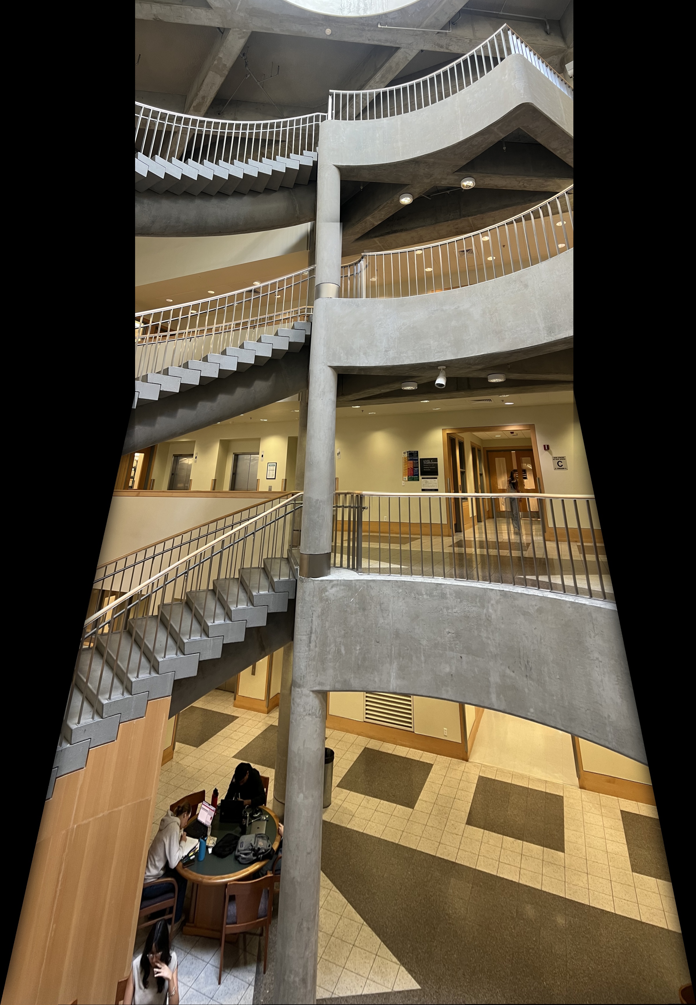
Example 3
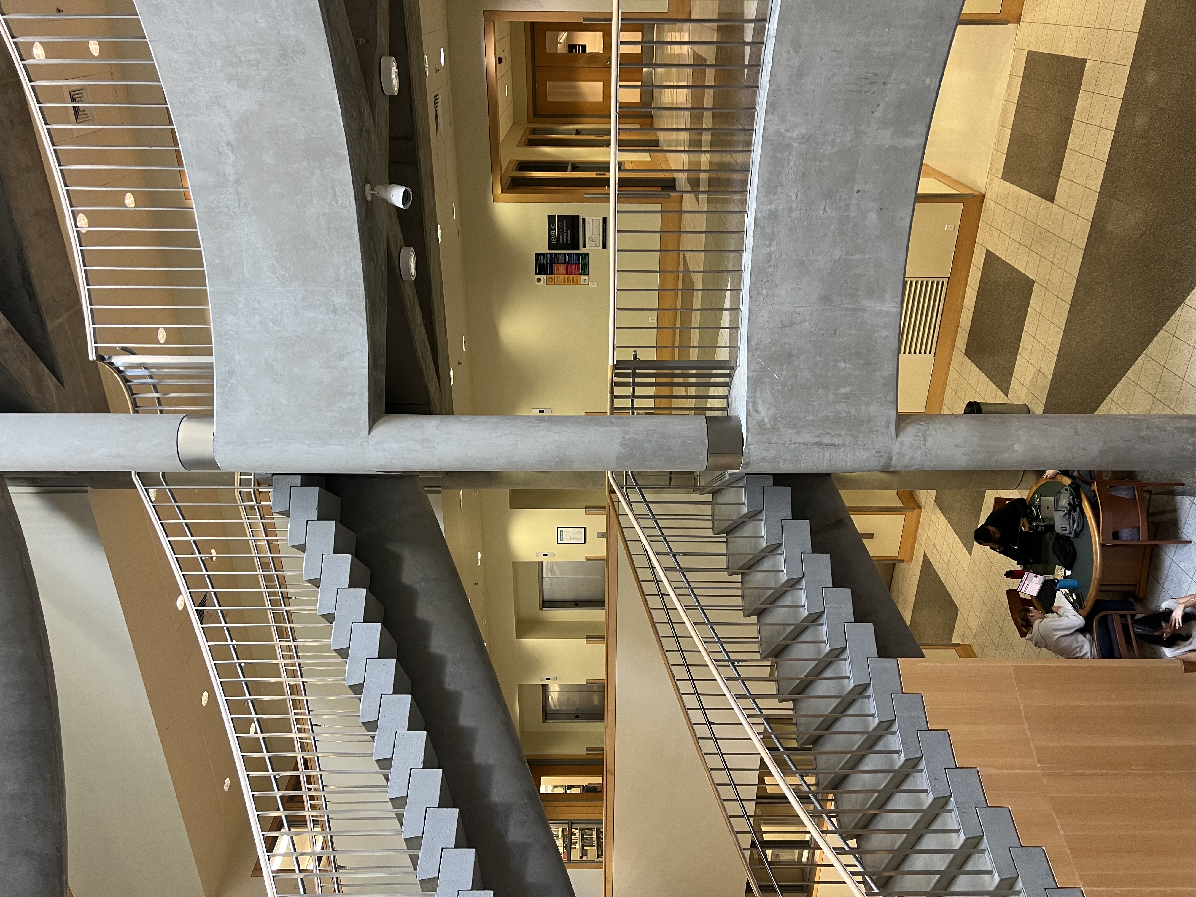
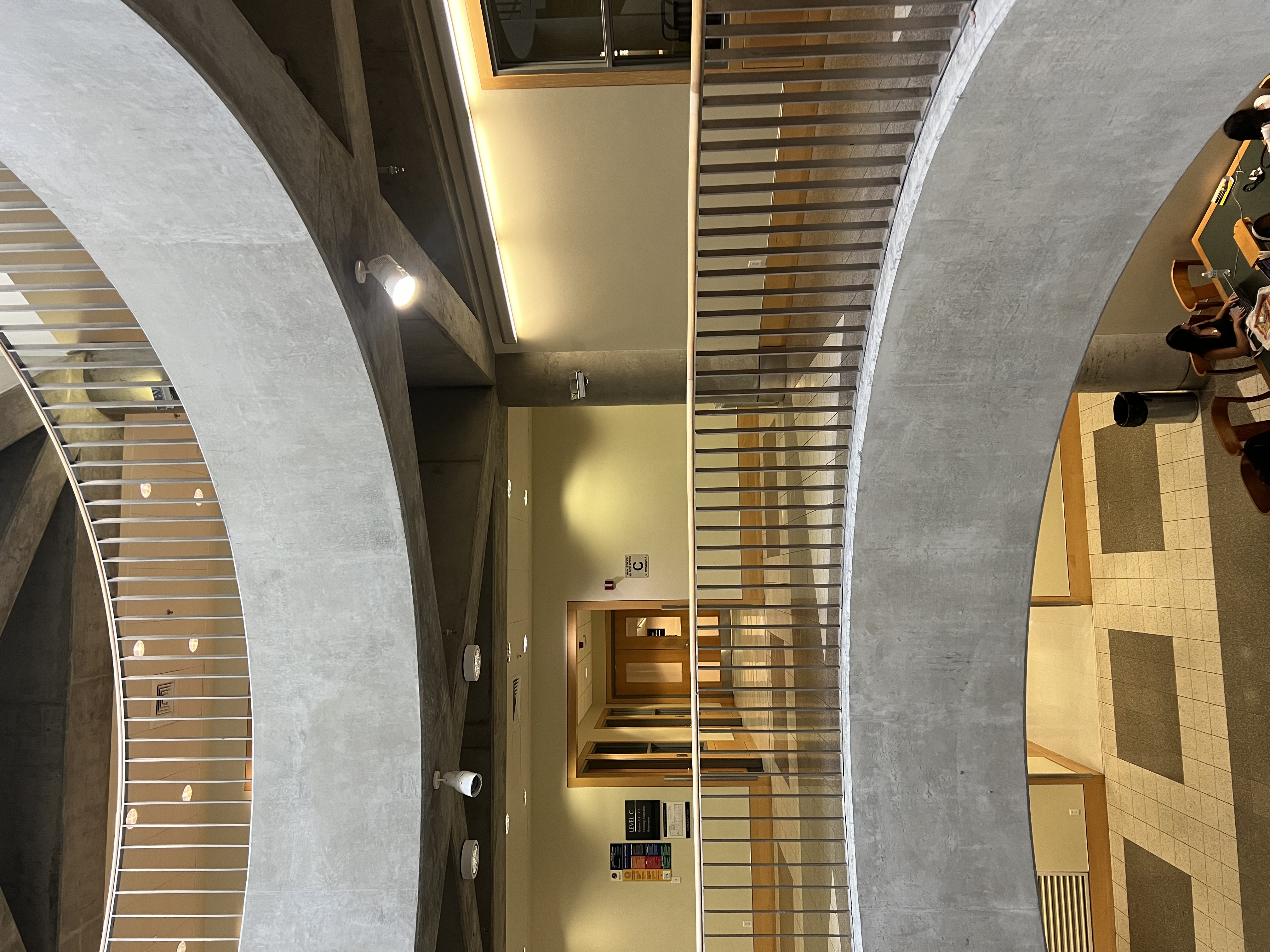
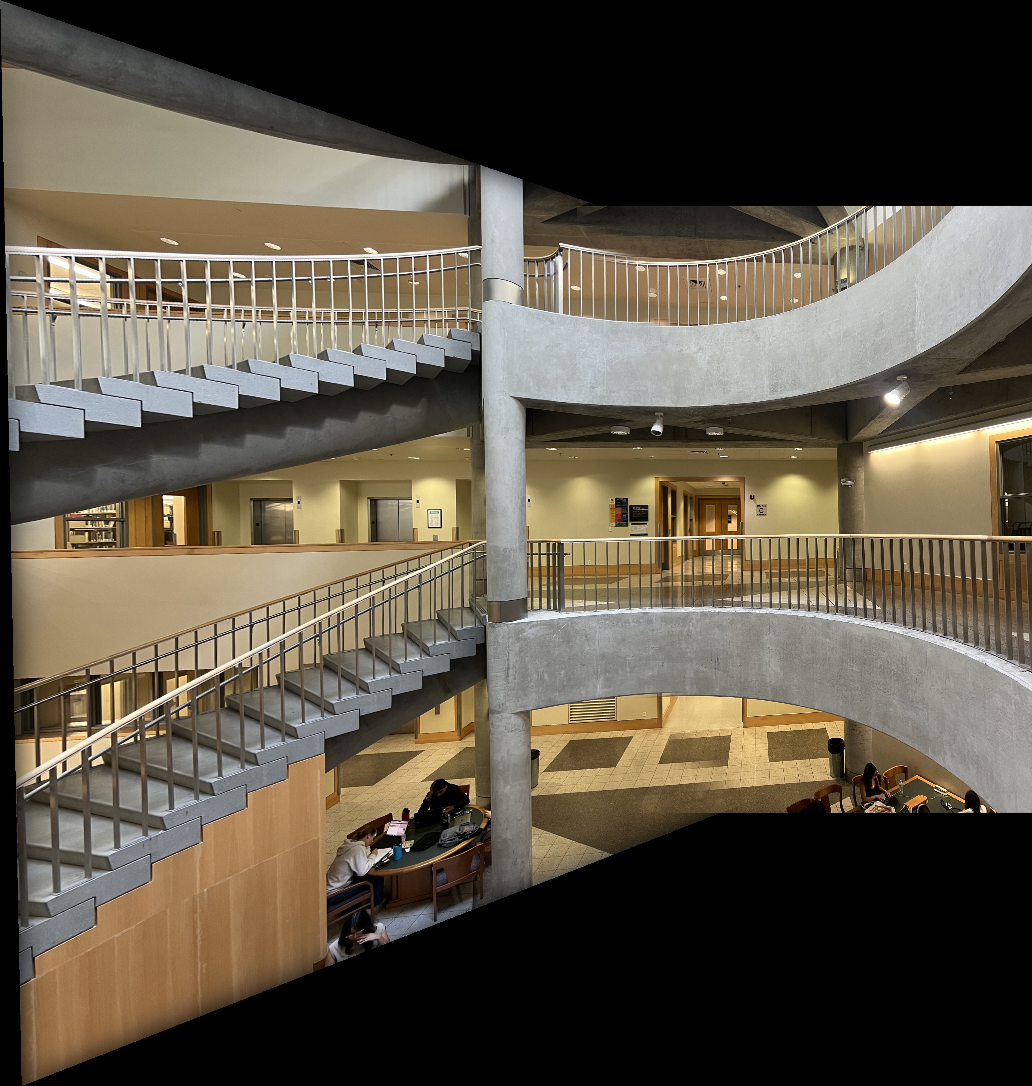
Example 4
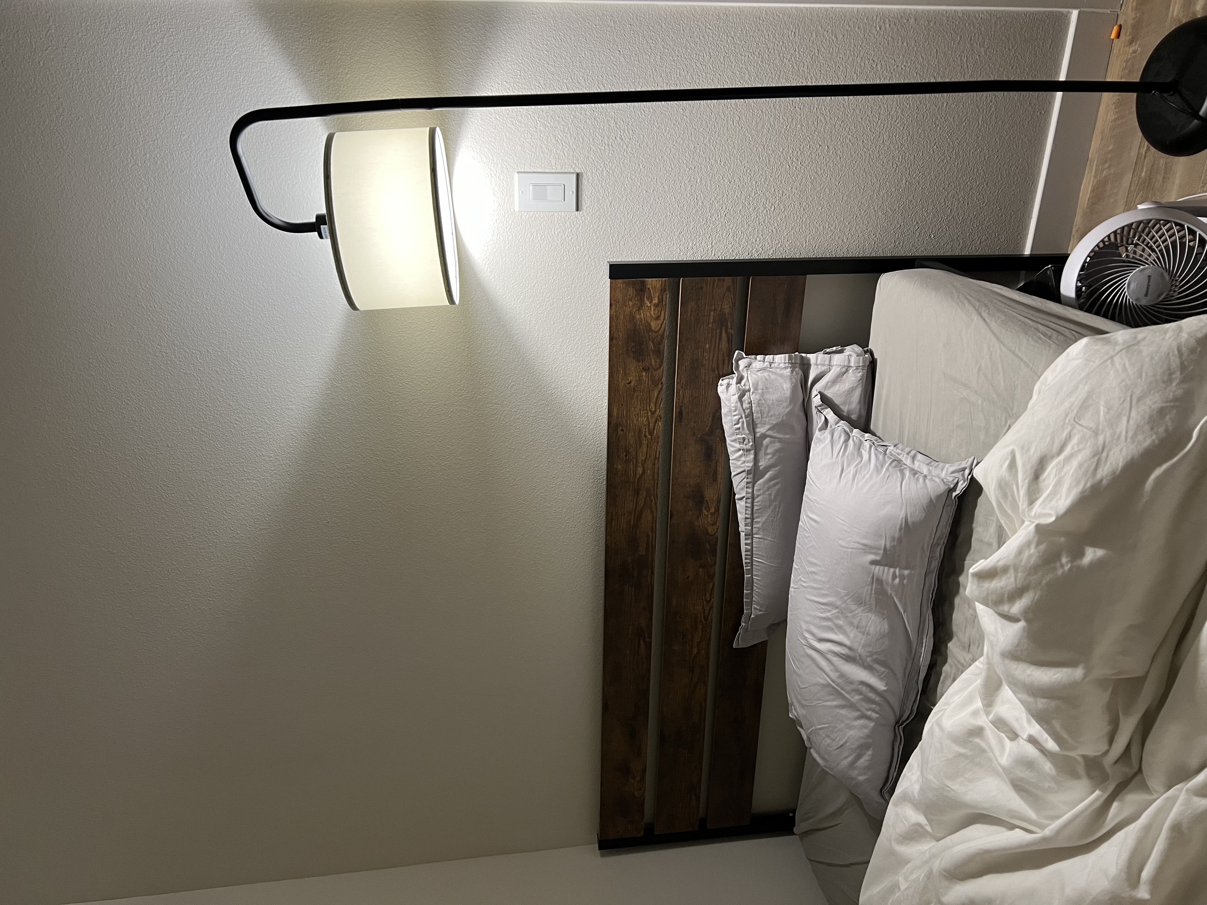
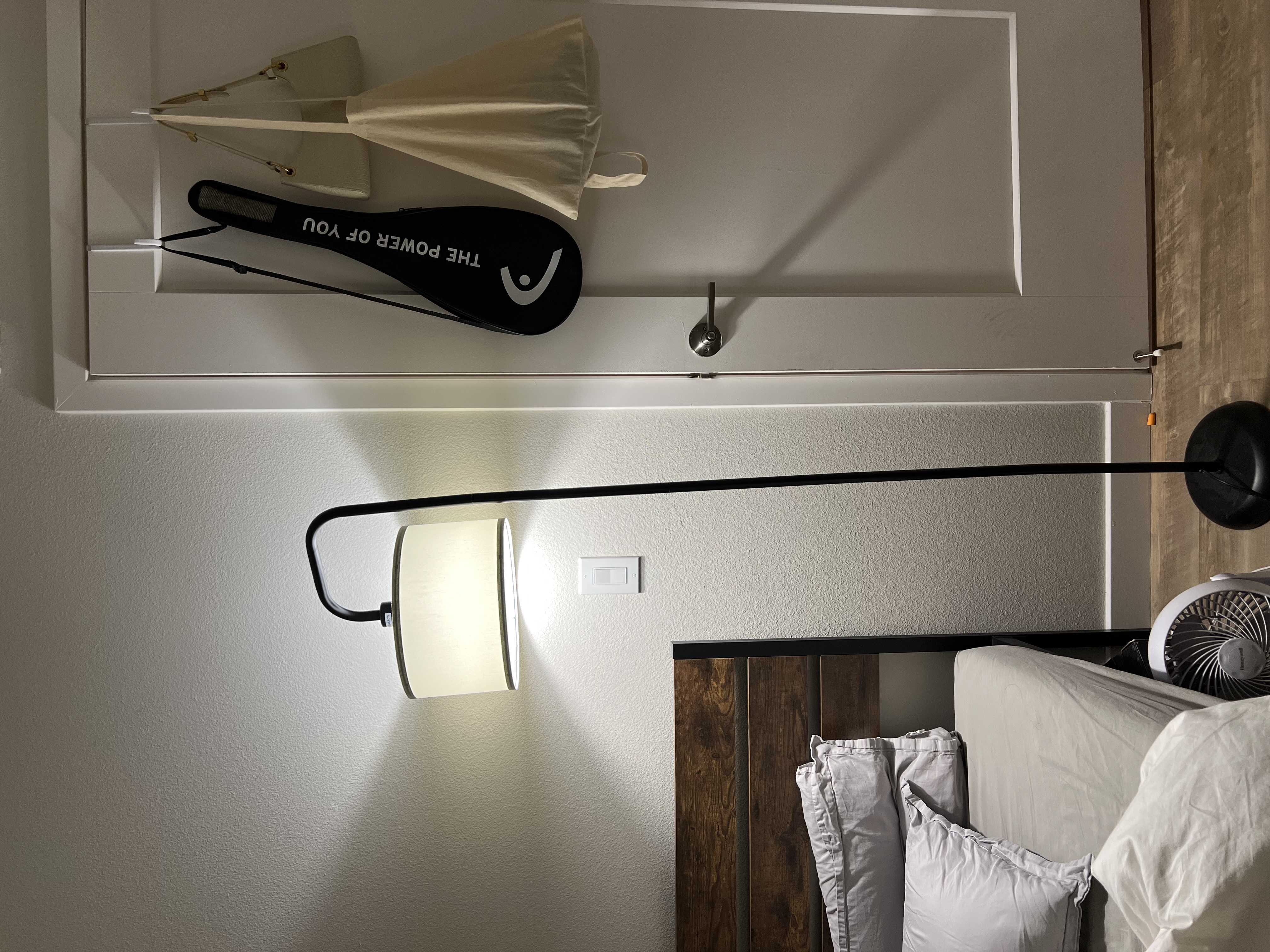
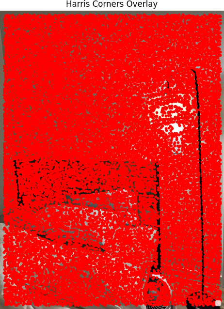
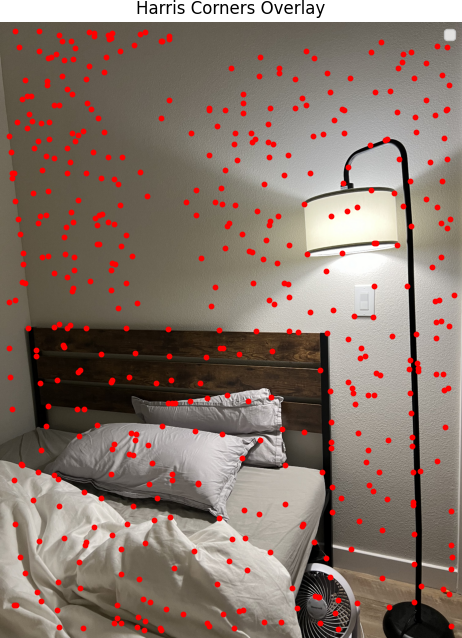
To begin, we locate potential interest points using the Harris Corner Detection algorithm. The Harris detector identifies corners by examining local changes in image intensity around each pixel, aiming to find points where intensity changes significantly in multiple directions. Such points are typically located at the intersection of two edges, making them ideal for feature matching. The function get_harris_corners is used to detect Harris corners in a grayscale image, returning both the Harris response values for each pixel and the coordinates of the detected corners.
Since the algorithm initially detects too many interest points, I employed the Adaptive Non-Maximal Suppression (ANMS) algorithm to eliminate clustered points and retain only the most significant, evenly distributed interest points. In ANMS, I iterated over all interest points and calculated the suppression radius for each point to its nearest stronger neighboring corner. After the iteration, the interest points were sorted by their suppression radius from largest to smallest, and the top n (where n = 500) points were selected as the final set of interest points. The purpose of ANMS is to retain interest points that are strong and have no significantly stronger neighbors nearby, resulting in a large suppression radius. These points are not clustered near other strong corners. In contrast, weaker corners near stronger neighbors have a small suppression radius and are thus discarded.
After identifying the interest points, I extracted an axis-aligned feature descriptor for each point by taking a 40x40 patch centered on the interest point and downsampling it to form an 8x8 descriptor patch. Using the rescale function from the skimage library, the 40x40 patch is automatically sampled to an 8x8 output with even spacing (s = 5), applying Gaussian blur to reduce potential aliasing. After sampling, each descriptor is normalized to ensure invariance to affine intensity changes.
To match feature descriptors between two images, I identified the best and second-best matches from the target image for each feature descriptor in the source image using L2-distance. Then, I applied Lowe's ratio test, comparing the ratio of the nearest neighbor distance to the second-nearest neighbor distance. Matches with a Lowe's ratio < 0.5 were retained as valid matches. This ratio test helps filter out poor matches by ensuring that the best match is significantly closer than the second-best match, thereby improving the robustness of the matching process.
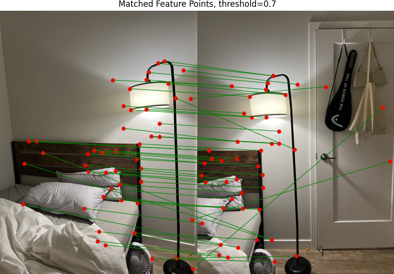
The sets of matched feature points using threshold=0.5 are more accurate than with threshold=0.7.
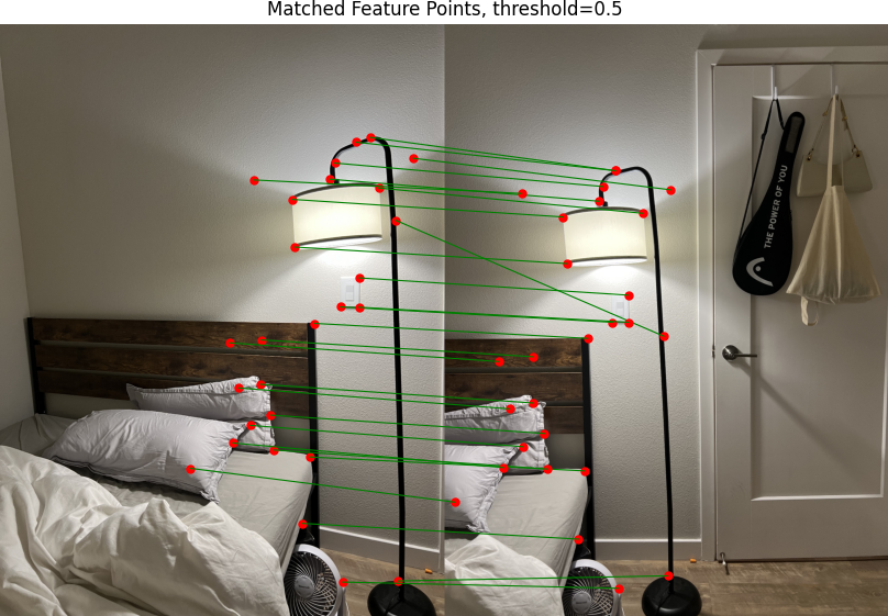
To find the optimal homography matrix that aligns the source image to the target image, the RANSAC algorithm follows these steps:
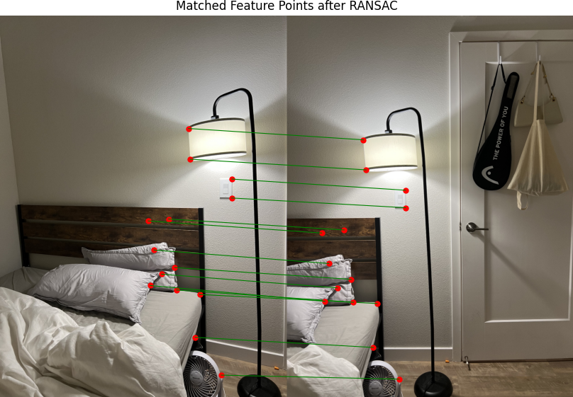
The largest sets of inliers are 7 for this example, and they are all accurately matched to the target interest points.
After obtaining the homography matrix, the mosaic from the two images are produced following the same steps from part A.
Example 1

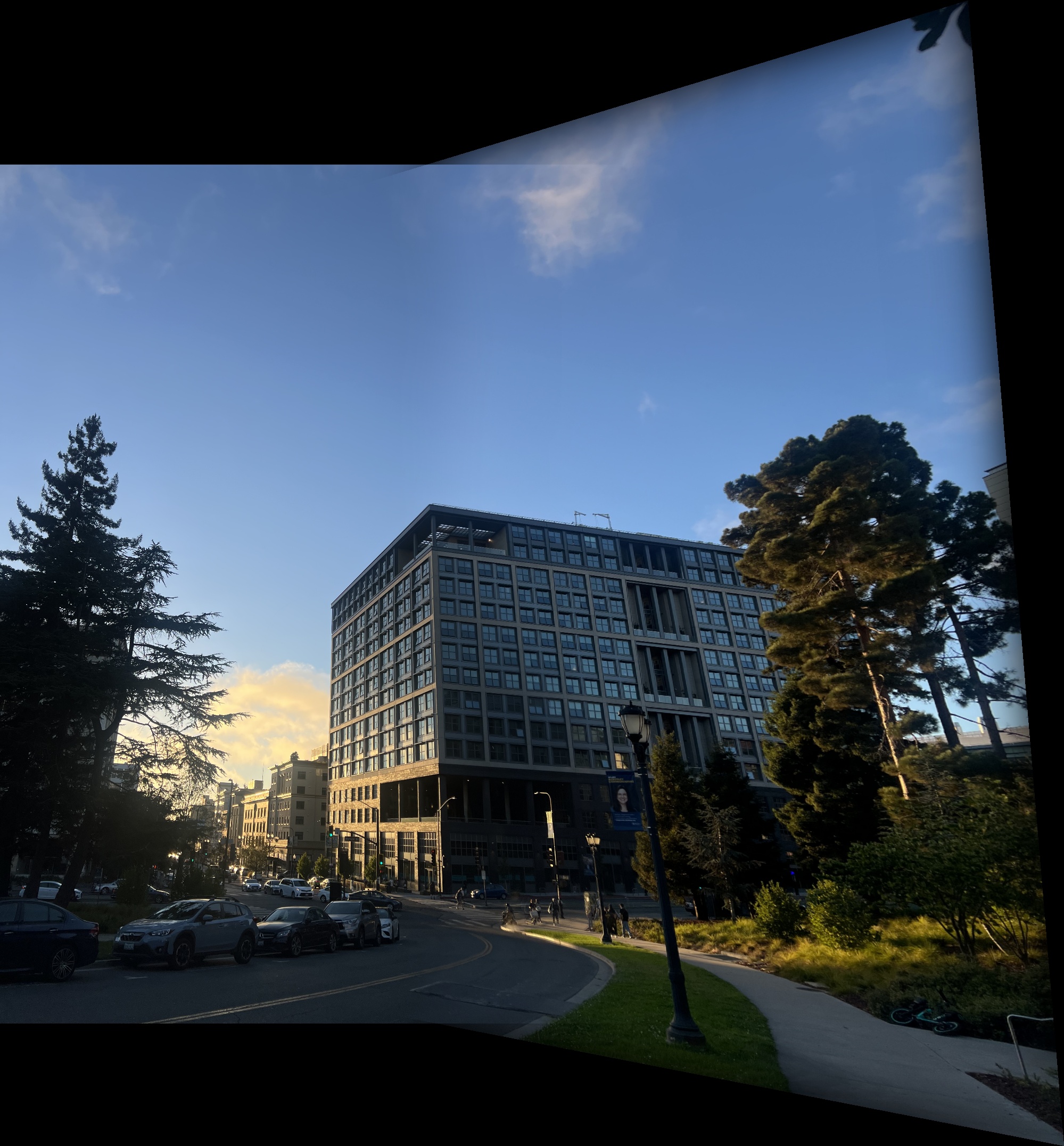
Example 2

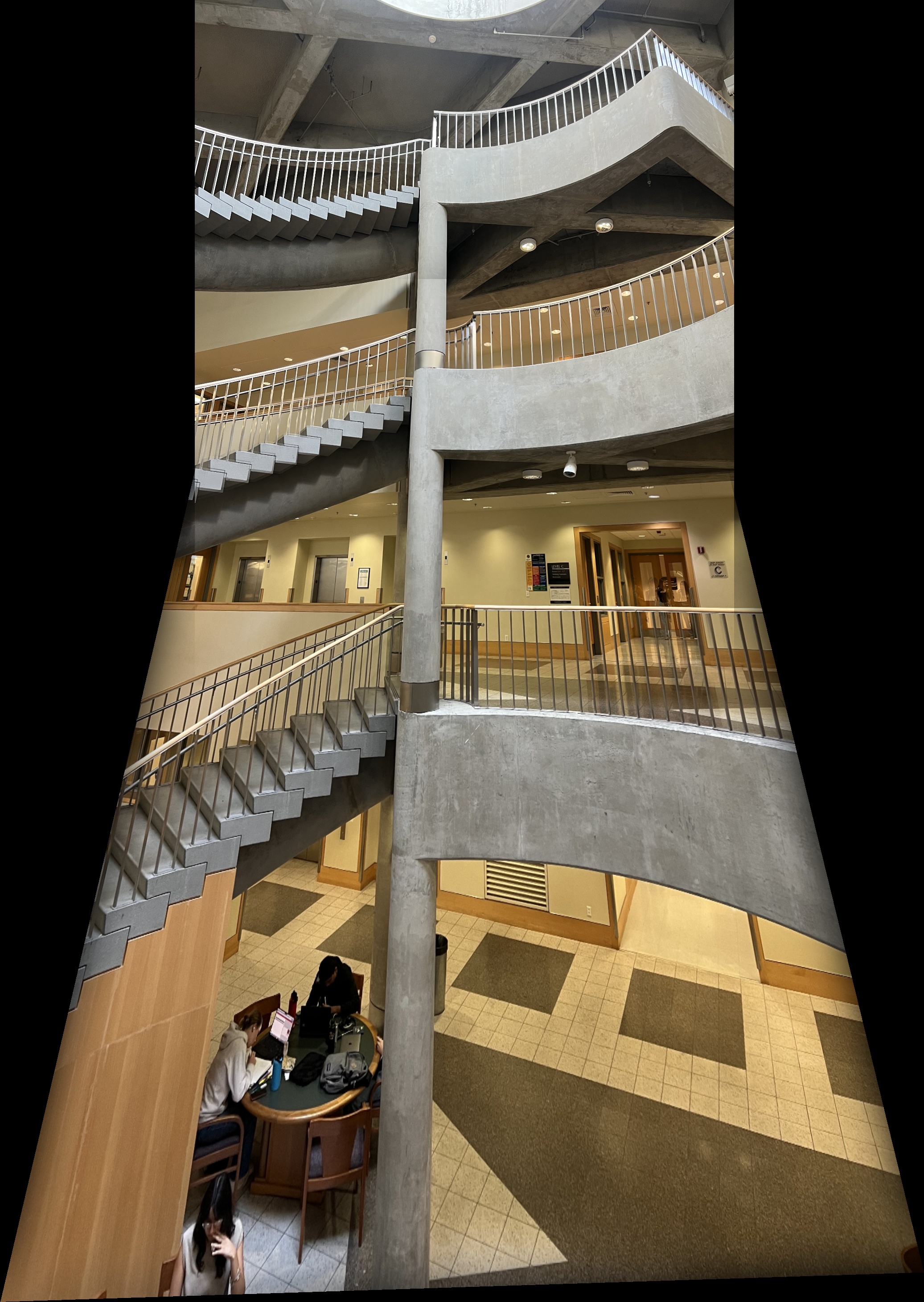
Example 3

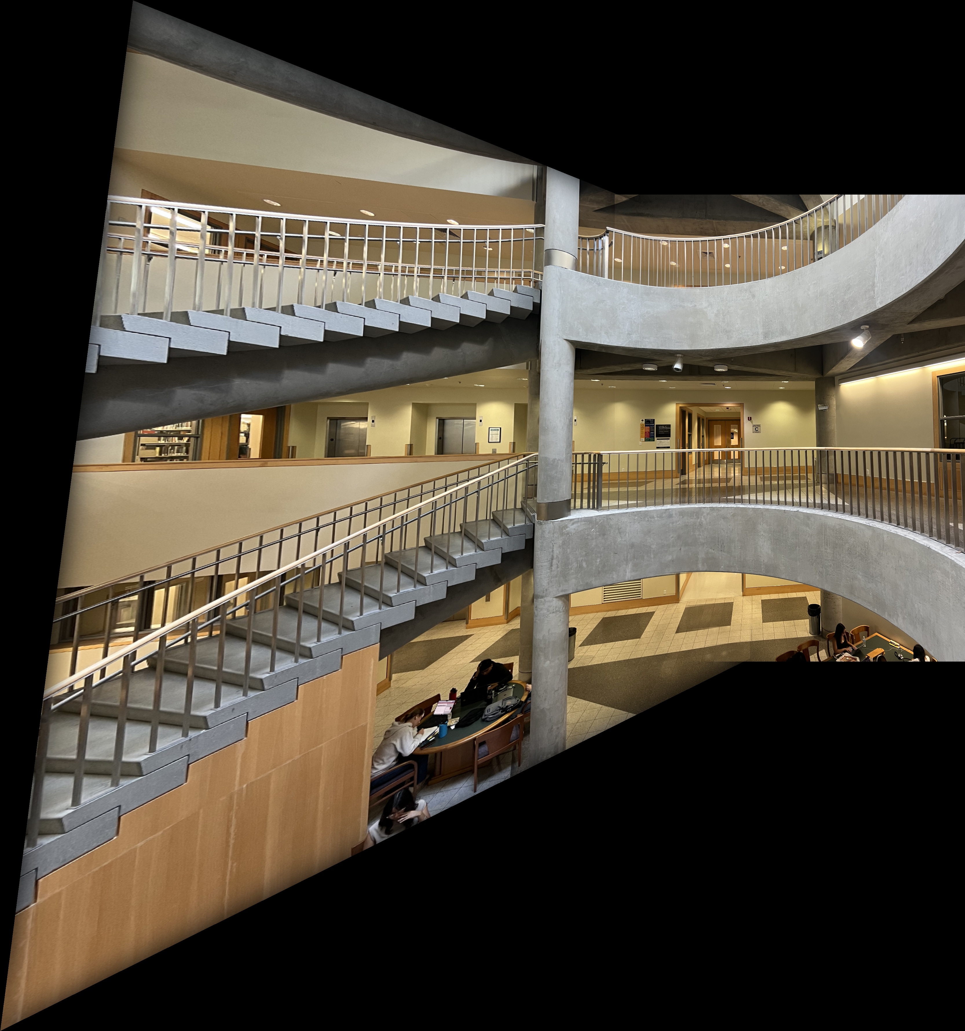
Example 4

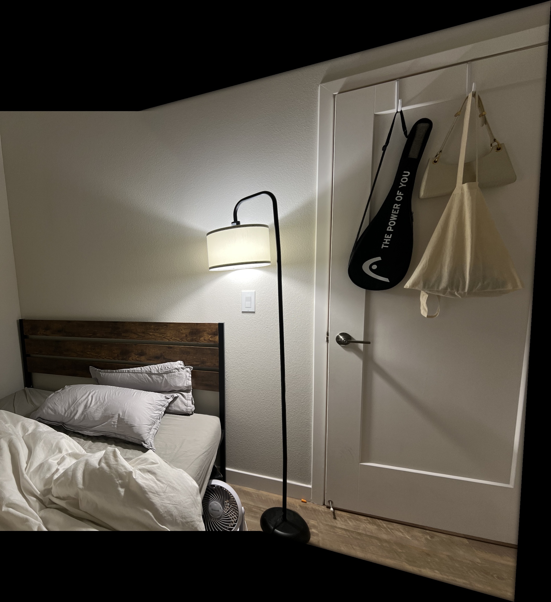
I learned how robust ANMS and RANSAC are in identifying strong interest points and accurately matching corresponding points for calculating the homography matrix. ANMS efficiently filters and distributes key points, while RANSAC reliably handles outliers to find the best transformations, making these algorithms powerful tools for precise and resilient feature matching in computer vision.